Visualisation of board game categories

mrpantherson has recently updated a collection of board game information from Board Game Geek and hosted in as Board Game Data - March 2017 on Kaggle.

Context of the data-set:

Being a fan of board games, I wanted to see if there was any correlation with a games rating and any particular quality, the first step was to collect of this data.

Content of the data-set:

The data was collected in March of 2017 from the website https://boardgamegeek.com/, this site has an API to retrieve game information (though sadly XML not JSON).

The are several interesting things about the data-set, and I thought the most straight-forward would be a simple visualisation exercise to examine what are the most common categories for the games. This script is thus a simple visualisation exercise to determine the most common categories in the data-set, using wordcloud and with standard barplot.

First off, some housekeeping lines for any R-script I work on:

## loading R packages
libs <- c("plyr", "dplyr", "tidyr", "ggplot2", "wordcloud", "mgcv")
invisible(lapply(libs, require, character.only=TRUE))
rm(libs)

# input data
file <- "https://raw.githubusercontent.com/minerva79/woodpecker/master/data/bgg_db_2017_04.csv"
df <- read.csv(file)

Since a game can be categorised into different genre, let’s treat the entire category as a standalone character vector, split them by , and remove leading and trailing white spaces.

## Date treatment of category
category <- df$category %>%
  as.character %>%
  lapply(., strsplit, ",") %>%
  unlist

## trim leading and trailing white spaces
category <- category %>%
  gsub("^\\s+|\\s+$", "", .)

Next, let’s construct a data frame based on frequency in which the different type of categories:

cat_dat <- data.frame(table(category))

Let’s visualise the frequency with a simple wordcloud

pal <- brewer.pal(9, "BuGn")
pal <- pal[-(1:2)]

wordcloud(cat_dat$category, cat_dat$Freq,
          scale=c(5,.2), min.freq=50, max.words=Inf,
          random.order=TRUE, rot.per=.15,
          colors=pal, vfont=c("sans serif","plain"))

Files in working directory

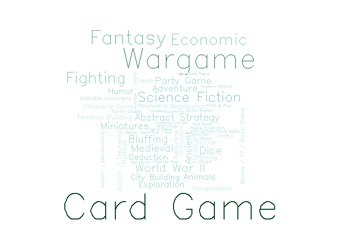
Seems that card game is the most popular category of board game, followed by wargame and fantasy.

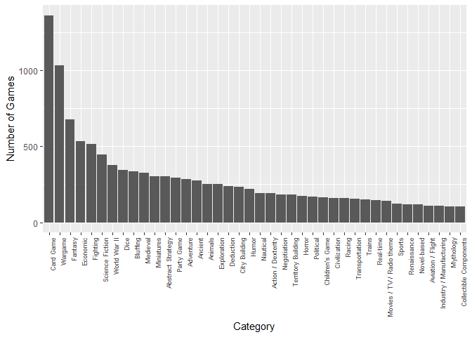
Let’s have another look at the top categories (i.e. categories that appeared in at least 100 games):

cat_d2 <- cat_dat %>%
  arrange(desc(Freq)) %>%
  filter(Freq >=100)

cat_d2$category <- cat_d2$category %>%
  as.character %>%
  factor(., levels=.)

ggplot(cat_d2, aes(category, Freq)) +
       geom_bar(stat="identity") +
       theme(axis.text.x = element_text(size=7, angle = 90, hjust = 1)) +
       ylab("Number of Games") +
       xlab("Category")

Files in working directory

So is there any correlation between category and sales?

# max number of categories listed for a game:
sapply(df$category %>% as.character, function(x) strsplit(x, ",") %>% unlist %>% length) %>% max

## [1] 11

df2 <- df %>%
  separate(category, paste0("V", sprintf("%02d",1:11)), sep=",") %>%
  select(game_id, V01:V11) %>%
  gather(var, category, -game_id) %>%
  mutate(category=  gsub("^\\s+|\\s+$", "", category)) %>%
  select(-var)

df2 <- df2 %>%
  left_join(df %>% select(game_id, owned))

df3 <- df2 %>% filter(category %in% levels(cat_d2$category)) %>% mutate(category = factor(category, levels=levels(cat_d2$category)))

ggplot(df3, aes(category, owned)) +
  geom_bar(stat="identity") +
  geom_line(data=cat_d2, aes(x=as.numeric(category), y=Freq*2000), stat="identity", colour="blue") +
  scale_y_continuous(sec.axis = sec_axis(~./2000, name="Number of Games")) +
  theme(axis.text.x = element_text(size=7, angle = 90, hjust = 1)) +
       ylab("Number of Copies Owned") +
       xlab("Category")

Files in working directory

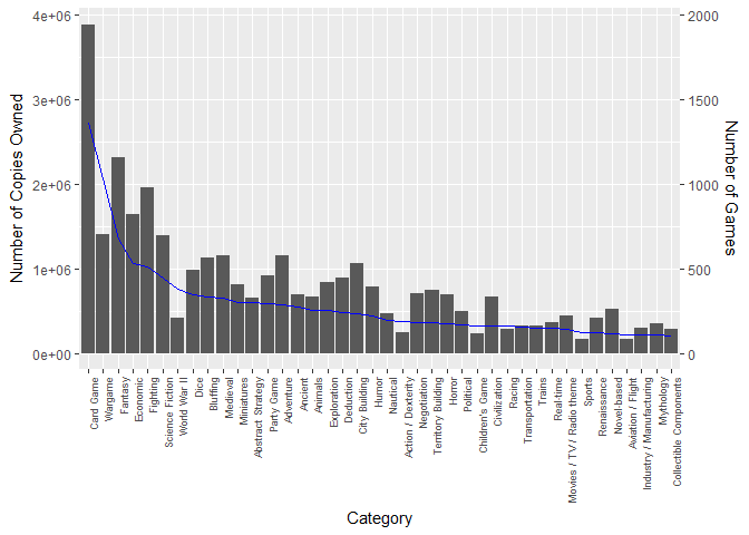
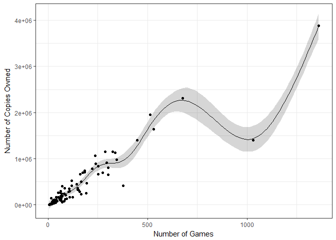
Seems like ownership of card games and the number of games seems to be high in both cases. However, that relationship doesn’t hold against other categories. To illustrate this non-linear relationship, here’s a simple plot of number of copies owned against the total number of games for each category:

df4 <- df2 %>%
  group_by(category) %>%
  summarise(owned=sum(owned)) %>%
  left_join(cat_dat) %>%
  na.exclude

fit <- gam(owned ~ s(Freq), data=df4)
newdat <- data.frame(Freq = seq(min(df4$Freq), max(df4$Freq), length=100))
newdat[, c("fit", "se")] <- predict(fit, newdata=newdat, se=T)[1:2]

ggplot(newdat, aes(Freq, fit)) +
  geom_line() +
  geom_ribbon(aes(ymin=fit-1.96*se, ymax=fit+1.96*se), alpha=.2) +
  geom_point(data=df4, aes(y=owned)) +
  ylab("Number of Copies Owned") +
  xlab("Number of Games") +
  theme_bw()

Files in working directory

Written on April 29, 2017